Navigating Through the Ranks

In the September newsletter, I briefly described the reasoning behind why environmental professionals would choose to employ the Toxic Equivalency Quotient (TEQ) approach to a contaminated site. My goal was to get your attention as to how this method can be a powerful tool that can be used to focus the chemical scope of the initial phases of an investigation, given that enough prior toxicological research has been conducted to statistically weight each member of the chemical group in question. I ended the last edition with an illustration showing how vastly different the final TEQ values can be, depending on how the data user assesses the value of each non-detected (ND) analyte within a sample. In this edition I will demonstrate a mechanism that is originally borrowed from the fields of biological and industrial statistics for calculating the means for censored or ND data, the Kaplan-Meier (KM) method.

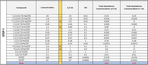
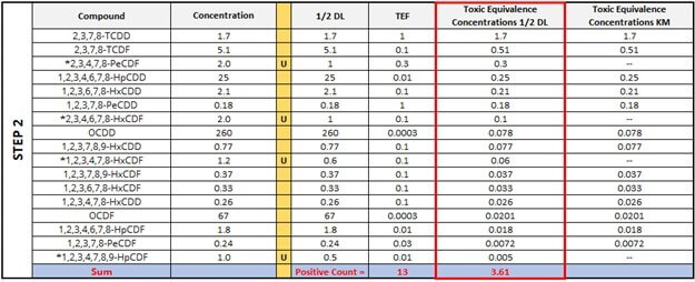
As a refresher, Step 1 is a demonstration of how different the overall TEQ values can be in each sample depending on whether ½ of the detection limit (½ DL) is substituted for the ND values or “0” is used instead. Step 2 simply ranks all congeners from largest to smallest (17 to 1) using the Toxic Equivalence Concentration ½ DL column. Notice how we are including those that are ND. As we introduce the TEQ KM values, we will now demarcate the ND values as null values, or absent; all the while, maintaining their rank alongside the standard toxic equivalency concentrations (TECs). This will become important later.

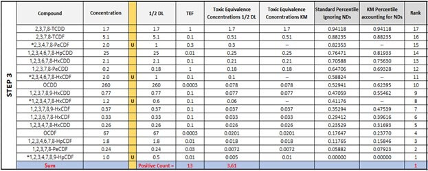
Now, Step 3 will introduce percentiles, which will be calculated differently (according to the Standard Substitution method or the KM method) depending on whether we allow the ND values into the calculation or not. Even though the Standard Substitution method does not necessitate the calculation of percentiles, the table below includes them in order to show where the ND values would be ranked in the KM method. For the first two congeners, 2,3,7,8-TCDD and 2,3,7,8-TCDF, the percentiles are the same. However, notice what happens to the percentile in the KM column as we move down to Rank 14 with the red arrow. As this method computes percentiles only for detected observations, the number and position of NDs influences the percentiles calculated for those observations that were detected at a rank less than the current position. Therefore, the percentiles for congeners with the rank of 14, 13, 12, and so on, are greater from the KM Percentile column except for Rank 1, which is automatically 0.

When the KM Percentile column is scrutinized, we can see that for the highest ranking value of 1.7, there are 17 values at or below it, with 16 below, so the calculation for the percentile is 16/17, or 0.94118 specifically. This is appropriate, insofar as the 4 ND values are all below a detected 1.7. The second-highest detected value is also identical to the Standard Percentile, and so the calculation for this position is 15/16 * the previous higher KM Percentile (0.94118), or 0.88235. The third highest value is a ND value at < 0.3. Its position relative to all values below 0.3 cannot be known, so a percentile is not calculated at this point even though the effect of this vacancy will be recognized in the percentiles with ranks below it. Rank 14 is a point of departure between the 2 methods as this position displays a greater percentile for the KM method when compared to the Standard Substitution method. This is because the KM Percentile = 13/14 * the previous higher KM Percentile of 0.88235 from Rank 16 instead of the absent value for Rank 15. This pattern for the KM Percentile to be greater than the Standard Percentile will cascade downward to all other ranks below, with the final exception of the rank of 1. With the correct KM Percentiles in place, now we will imagine the data being drawn in the form of a histogram, with the length being the Toxic Equivalence KM value and the width of each detected congener being represented by a new ‘adjusted’ percentile as being described as the amount of percentile being taken up by the rank. Another way of defining the ‘adjusted’ percentile is the difference between the next highest percentile and the current percentile. A partial description of the calculations is listed below with a final table that presents the final KM TEQ value. (Toxic Equivalence Concentration KM) x (Difference in KM Percentile) = Length x Width

- Rank 17 “Area” of histogram = (1.7) * (1 – 0.94118) = 0.100
- Rank 16 “Area” of histogram = (0.51) * (0.94118 – 88235) = 0.030
- Rank 15 is not calculated.
- Rank 14 “Area” of histogram = (0.25) * (0.88235 – 0.81933) = 0.01576

▼

- Rank 1 “Area” of histogram = (01) * (0.07923 – 0.0) = 0.00079

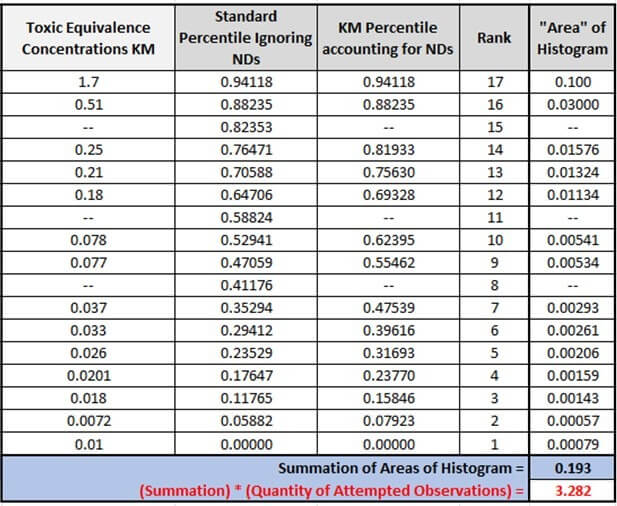
Note: Even though the underlined value in Rank 1 was ND, it is forced into the KM mechanism by Efron’s bias correction – stating that the lowest value should always be considered positive.

If we revisit the first two examples using the standard substitution method from Step 1, the decision of whether to use “0” or ½ the detection limits is critical. The percent difference between the outcomes of these two methods is 12.9%, and it would be higher still if the full amount of the detection limits were used for the substitution.

In this case, the KM method provides an option for calculating TEQs in data sets that withstand the potential data variance that can result from amassing historical data from key regions in a site cleanup. Oftentimes, it is necessary for consultants and engineers to acquire vast amounts of historical laboratory data from past time periods in which they were not the primary contractor, and they did not have control or influence concerning what substitutions were used in the TEQ calculations; or worse yet, they may be forced to use TEQ historical data in which a portion of the data set used 0 and another portion of the data set used ½ DL. In cases like this, the KM method can provide comparability and clarity when looking into the past through an analytical lens.

However, there are key necessitating factors that must be taken into account in order for the KM method to be used, and they need to be taken into careful consideration when employing the method.

Firstly, the method falls short of reliability if and when all ND values calculate out to have only one threshold, or to put another way – if all the ND values, multiplied their appropriate toxic equivalency weighting factors (TEFs) all are represented by the same number. This is unlikely in the case of computing total TECs, because the thresholds for different congeners are computed by multiplying the detection limit by the TEF, which differs for different congeners. Another problematic situation occurs when a high ND value for a high-toxicity congener such as 2,3,7,8-TCDD presents a TEC value that is higher than all TECs from detected concentrations. In this situation, no calculation procedure can give a reliable estimate of the total TEC because the KM method will ignore this high TEC ND, because it has no information content. A lower detection limit must be implemented before reliable estimates of the total TEC can be made using any calculation method. In this situation it may be necessary to substitute the detection limit in order to provide a worst-case value for the total TEC, taking into consideration that the real TEQ would be lower.

I hope that I have provided some insight and perhaps sparked some interest in looking at different ways to calculate TEQs and consolidate efforts to glean substantive toxicological information from using just one or two analytical methods. I believe that the near future is sure to bring more knowledge of familial chemical groupings, analytical methods, and statistical methods that take the underlying concept of the TEQ further into realms not yet thought of.

MARK LYBEER

DATA PROJECT MANAGER

References

Helsel, Dennis R. Summing nondetects: Incorporating low-level contaminants in risk assessment. Integrated Environmental Assessment and Management, July 2010, Vol 6; Issue 3. 2009.

Wheeler, Richard (2007). Benzopyrene DNA adduct 1 JDG.png, Zephyris, Online image.

Washington State Department of Ecology; Toxics Cleanup Program (2007). Evaluating the Toxicity and Assessing the Carcinogenic Risk of Environmental Mixtures Using Toxicity Equivalency Factors. Supporting material for Cleanup Levels and Risk Calculation (CLARC), October 2007.